Excel Error and Error Handling Roundup

Excel Error and Error handling Roundup 

Technology used: Office 365, Excel 2021

You just typed the closing parentheses of that powerful lookup formula that’s going to save you hours next month on the report. You slowly depress the Enter key while feeling empowered as if the Excel gods have chosen you! Feeling the click your stomach turns as you watch the fire bestowed upon you turn into a ball of steam that wisps away.  Excel is taunting you. Instead of the sales figures, you see #N/A but what could be wrong? 

Excel’s formula errors are unpleasant to see but they’re trying to help us improve our spreadsheet game. In this article, we’ll learn about the types of formula errors that Excel will display, a few formulas to help us avoid them and some thoughts on good use of error trapping. 

What are formula errors

Formula errors are the result that Excel returns when it is unable to evaluate and provide a proper answer to the formula in the cell. The errors always begin with a number sign (i.e. #) and then a word to give you a clue as to what is causing the error. Below is a table listing common errors and some of their causes

Error (As shown in the cell)Description
#N/ACommonly found in lookup formulas (e.g. Vlookup, Hlookup, Index, Match, etc) if the formula is unable to find what the formula is looking for
#VALUE!Excel’s general error. Simply put, something is wrong with the formula.
#REF!A cell reference is invalid, typical if you delete a row/column that was being referenced by the formula
#DIV/0!Division by zero. The result of which is undefined mathematically
 #NUM!Mathematical operations are being applied to non-numeric cells. You can force text to be treated as numbers using the VALUE() function.
#NAME?Excel doesn’t recognize the formula name, usually the result of a typo (e.g. =SMU(A1:A5) instead of =SUM(A1:A5)
#NULL!The range is not constructed correctly in the formula’s parameters (e.g A5 B7 instead of A5:B7)
#SPILL!Excel is unable to return the results because there isn’t enough room. For example a FILTER function is returning 10 results but there are only 9 blank cells available
Microsoft Excel’s Formula Errors

What formulas can be used to stop errors? 

Excel gives us two formulas to handle or trap errors. Using these formulas can make your worksheet more robust and user friendly. They can also allow your workbook to function despite Excel being unable to calculate a cell. 

IFError

The IFError function allows you to provide an alternate value or formula if Excel encounters any of these errors:  #N/A, #VALUE!, #REF!, #DIV/0!, #NUM!, #NAME?, or #NULL!.

Its usage is: 

=IFError(cell reference or formula, value if error

The cell reference is any cell or formula that you are testing to see if it has or results in an error.  

The value if error is what will result if there is an error. Here you can be really creative. A common usage would be a helpful error message consider something like: 

=IfError(1/0, “Division by zero is undefined”)

In this case the formula 1/0 (e.g. One divided by 0) would result in #DIV/0!, we can replace that with the more friendly error message explaining that we can’t divide a number by zero. 

But you can also use a substitute formula. For example:

=IFError(1/0, A1/B1)

This formula will result in the value of cell A1 divided by B1. Coincidently if the values of A1 divided by B1  would result in an error, then that error will be displayed. 

Using the IFERROR formula gives us a lot of flexibility in trapping and resolving errors. 

IFNA

IFNA works very similar to IFERROR except it only works with the #N/A error. Otherwise it’s usage is identical. Recall from the table above that the #N/A error is only encountered with lookup formulas thus this formula will only trap cases where the lookup value can’t be found in the table. 

Its usage is:

=IFNA(Cell Reference or Formula, value if error

For instance:

=IFNA(Vlookup(A1,A2:B20,2,FALSE),”Value was not found”)

Would display Value was not found instead of #N/A if the lookup value couldn’t be found. 

Similar to IFERROR you can use a formula or value in place of the value if error parameter, this can help keep the logic of your workbook functioning.

Consider this example:
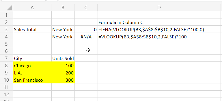
A Vlookup function encapsulated by an IFNA function

As you can see, since New York is not in the list an #N/A is triggered, the first version of the formula returns a 0 which we could then use in our workbook if we need to. 

Trap every error? 

As you’re building your workbook consider the effects of trapping the error versus knowing there is an error. Sometimes we want to see the error, to know that the workbook is not working as we intended. For instance in the example above, we are returning 0 for cities not in the list, however since our worksheet is to tell us total sales $0 is also an acceptable answer. We have no easy way to tell if there were no sales in a city or that the city is not in the list, which might indicate a data issue. 

This is a problem known in Computer Science as the semi predicate problem where an error can be confused as a valid value. To prevent this care must be used when selecting what errors we want to trap and which we want to allow to break the workbook. 

Excel has a variety of error codes to help the user understand why their formula isn’t working. Excel also has useful formulas for trapping and resolving potential errors. Careful and considerate use of these can lead to well constructed and robust workbooks. 

Do you want to learn how to automate your financial workpapers? Do you want to get started with VBA?

My book, Beginning Microsoft Excel VBA Programming for Accountants has many examples like this to teach you to use Excel to maximize your productivity! It’s available on Amazon, Apple iBooks and other eBook retailers!

Learn More:

Function pages on Microsoft Support
IFNA

IFERROR

#VALUE Error

#NUM! Error

#NAME? Error

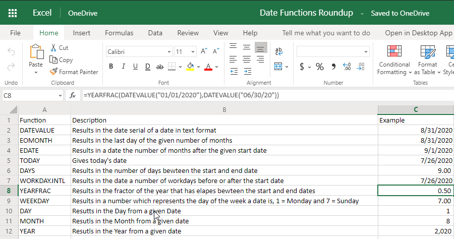
Microsoft Excel Date Functions Round Up

What day is it? What day will it be 10 months from now? How many days until the end of next month? Microsoft Excel has a wide variety of date functions. This article will focus on several of the most useful. Hopefully you’ll find a few to add to your function repertoire.

Date Function

DATEVALUE

Excel stores dates in a serial number format. Serial number 1 represents January 1, 1900 and each day after that increments the serial number by one. In other words January 2nd 1900 is 2 and serial number 44074 is August 31, 2020. Most of the date functions require this serial number. If you want to work with a date in a common format such as 08/31/2020 DATEVALUE is your go to.

Usage is: = DATEVALUE(“date”)
Example: =DATEVALUE(“08/31/2020”) will result in its serial 44074

Note: For the examples in this article, we’ll use DATEVALUE in place of a date serial

EOMONTH

EOMONTH results in the last day of a given number of months. I wrote an entire post on it here already showing a use case in accrual accounting. You can read that post here.

Excel EOMONTH Function Leads to Consistent Expense Accruals

Usage is: =EOMONTH([DateSerial], [number of months])
Example: =EOMONTH(DATEVALUE(“08/05/2020”),0) results in 08/31/2020

EDATE

EDATE results in a date that is the specified number of months before or after the given start date. Use negative numbers to give prior months and positive values for future ones.

Usage is:=EDATE([start date], [number of months])
Example: if we want the following month =EDATE(TODAY(),1) or if we want the day one month prior =EDATE(Today(),-1)

TODAY

TODAY() results in today’s date, it can be used as a parameter in formulas that need a date and we’ll use it in many of the following examples.

Usage: =TODAY()
Example: to get today’s date =TODAY()

DAYS

DAYS results in the number of days between two dates, excluding the end date. Unlike other date functions you can provide a date in a text format as a parameter. Although it won’t hurt any if you use DATEVALUE, a serial date or even TODAY()

Usage: =DAYS([end date],[start date])

Example: to get the number of days between August 1st and August 10th =DAYS(“8/10/20”,”8/1/20”)

WORKDAY.INTL

WORKDAY.INTL results in the date that’s the number of weekdays away from the given start date. This version of the WORKDAY function allows finer control over weekends and holidays than the vanilla WORKDAY function. The weekend day combinations are listed in a table that can be found on Microsoft’s support page (links in the Learn More section at bottom). If the weekends parameter is omitted, the default weekend is Saturday & Sunday.

Usage: =WORKDAY.INTL([start date], [number of days, [weekends], [holidays])
Example: To get a day 5 workdays prior to August 1, 2020 where Wednesday is the only day considered a weekend: =WORKDAY.INTL(DATEVALUE(“08/01/2020”),-5,14)

YEARFRAC

YEARFRAC results In the fractional portion of a year that has(will) elapse between two dates

Usage: =YEARFRAC([start date], [End date])
Example:To see what portion of the year passes between January 1st and June 30th (i.e. 0.50) =YEARFRAC(DATEVALUE(“01/01/2020”),DATEVALUE(“06/30/20”))

WEEKDAY

WEEKDAY Results in a number which translates in the day of the week of the provided date.

A Result of 1 is Monday and 7 is Sunday the other numbers between Correspond to each successive day

Usage: =WEEKDAY([date])
Example: to find which day of the week (i.e. 7 which is Sunday) =WEEKDAY(DATEVALUE(“08/01/20”))

Extract functions

The next three are what I call the extract functions because they allow you to extract or single out a part of the given date.

DAY

DAY Results in the day portion of a given date. This formula is useful for extracting the day data when needed.

Usage:=DAY([date])
Example: to get the 1 out of August 1, 2020 =DAY(DATEVALUE(“08/01/2020”))

MONTH

Month results in the month portion of a given date. This formula is useful for extracting the month data when needed.

Usage: =MONTH([date])
Example: to get 8 (for August) out of August 1, 2020 =MONTH(DATEVALUE(“08/01/2020”))

YEAR

YEAR results in the year from a given date. This formula is useful but you need to extract the year from a given date.

Usage: =YEAR([date])
Example: to get 2020 out of August 1, 2020 =YEAR(DATEVALUE(“08/01/2020”))

Want to learn how to automate your financial workpapers? Do you want to get started with VBA?

My book, Beginning Microsoft Excel VBA Programming for Accountants has many examples like this to teach you to use Excel to maximize your productivity! It’s available on Amazon, Apple iBooks and other eBook retailers!

Learn More:

Function pages on Microsoft Support:

Example Workbook can be found at: MicroSoft OneDrive

N Function Allows for Documentation in Excel’s Formula Bar

Microsoft Excel’s N function has many uses, including Switching and in line documentation

We commonly use Excel’s comment or note function to explain formulas or where the cell values come from. But, have you ever wanted to put this information in the formula bar itself? Sometimes it’s more helpful to document our formulas and data right where the user is reading them. Enter Excel’s N function. 

The N function converts it’s parameter to a number. This is not to be confused with the VALUE function which converts text to number values. The N function will convert any text given to it to the value zero. If that doesn’t sound useful, keep in mind the additive property of zero anything added to zero is the original value. With this in mind, you can use this function to insert comments into the formula. For example if you had a formula to give an annual average and increase it by 3% your formula might be =AVERAGE(A1:A12)*1.03+N(“Returns a 3% increase in the average”). This use is shown in the featured image. 

Switching in Formulas 

Another interesting property of the N function is the way it converts TRUE or FALSE values. N will return the value 1 for a TRUE or 0 for a FALSE. Considering the multiplicative properties of 1 and 0 we can use this to create switches in our formula. A switch is where an operation is included in the final result if it’s multiplied by 1.  For Example, this formula would result in the value 2 =(2*N(FALSE))+(2*N(TRUE)) if you expanded it it would be (2 x 0) + (2 x 1), change the first FALSE to TRUE and the value will increase to 4. With some careful workbook design, the N function can be used to replace nested IF statements which would serve a similar purpose. Let’s look at a more sophisticated example. 

The sample workbook features quarter ending dates and the date of the current workpaper. By simply changing the workpaper date the Year To Date amortization updates appropriately. I’ve also used the comment N technique described earlier to demonstrate that use. 

The N function is deceptively powerful. On the surface it would be easy to dismiss, but with a little ingenuity and careful workbook design it’ll allow you to simplify your workpapers and provide great documentation in the formula bar. 

Do you want to get started with VBA? Want to learn how to automate your financial workpapers? 

My book, Beginning Microsoft Excel VBA Programming for Accountants has many examples like this to teach you to use Excel to maximize your productivity! It’s available on Amazon, Apple iBooks and other eBook retailers!

Download the sample workbook (Excel 2010 and higher):

Learn More: 

https://support.office.com/en-us/article/n-function-a624cad1-3635-4208-b54a-29733d1278c9

Raspberry Pi Cooling Test

Raspberry Pi Cooling Test

Dated: 8/1/2018 Technology/Software used: Raspberry Pi 3 Model B, Raspian Stretch (June 2018)

I’ve owned my Pi for a couple years now. I’ve always wanted to overclock it. Before you overclock you have to have a good cooling solution. I wanted to take this opportunity to test some various cooling solutions and talk about the process I went through. In this post I’ll explore my results from various cooling tests I conducted.

A word of caution: Overclocking your Raspberry Pi may void your warranty, do at your own risk. Due to differences in manufacturing some Pis may overclock well, some will not at all.
The following in no way is meant to be scientifically accurate testing and your results may very.

Why do I want to overclock? Well I sometimes use my Pi to run the RetroPie operating system. I enjoy retro gaming and I would love to be able to emulate N64 better. There’s a lot of mixed opinion and the general consensus is that the Pi is not fit for N64 emulation (spoiler alert: they’re right) but I wanted to try and see for myself if it was possible to play Goldeneye on my Pi.

Ultimately I wanted to use both a small 5 volt fan and heat sink. But I was interested in seeing the thermal performance of each component individually. I tested the heat and processor throttling of a stock configuration using the sysbench application. I was inspired by Christopher Barnett’s thermal tests on his YouTube channel – Explaining Computers and I used a similar bash script to test.

Moding the Case

My case, a very basic one for the Pi, wasn’t designed to hold a fan. I cut an opening and screw holes for the fan with a Dremel tool. You can see in the photos below the before and after. I hadn’t cut acrylic plastic before. I used a regular cutting disk for this. While it did the job, I noticed the plastic was getting a bit gummy which made it hard to control. I would have benefited form scoring the plastic before cutting. If I have to do this again, I’d try a different cutting disk and maybe first score the circle before cutting.

With the prep-work done I began the test. I tried five configurations, the Pi in the closed case (before cutting the fan hole), the Pi in an open case, the fan by itself, the heat sink by itself and finally both the heat sink and fan.

Before:

After:

Why is the cooling so important?

Running electrical components too hot can cause them to fail over time. Getting too hot in one instance can also cause an immediate failure. However, many modern computers have built in thermal protection which will reduce their power in an effort to cool the unit down. The Pi is no exception. Its thermal protection kicks in at about 80 C at this point the Pi will reduce it’s clock-speed to cool itself. I wanted to see how significant the throttling is. So I tracked both the average clock-speed throughout the entire test and the temperature between each test.

This is the script I had used. It’s a bash script which in Linux is like a batch file Windows. In other words a file which automatically runs a series of commands.

#! /bin/bash
echo "Baseline"
vcgencmd measure_temp
vcgencmd measure_clock arm
echo "Test 1"
sysbench --test=cpu --cpu-max-prime=20000 --num-threads=4 run >/dev/null 2>&1
vcgencmd measure_temp
vcgencmd measure_clock arm
echo "Test 2"
sysbench --test=cpu --cpu-max-prime=20000 --num-threads=4 run >/dev/null 2>&1
vcgencmd measure_temp
vcgencmd measure_clock arm
echo "Test 3"
sysbench --test=cpu --cpu-max-prime=20000 --num-threads=4 run >/dev/null 2>&1
vcgencmd measure_temp
vcgencmd measure_clock arm
echo "Test 4"
sysbench --test=cpu --cpu-max-prime=20000 --num-threads=4 run >/dev/null 2>&1
vcgencmd measure_temp
vcgencmd measure_clock arm
echo "Test 5"
sysbench --test=cpu --cpu-max-prime=20000 --num-threads=4 run >/dev/null 2>&1
vcgencmd measure_temp
vcgencmd measure_clock arm
echo "Complete"

The script will run the test five times. We’ll look at the specifics of the each command next, but in essence it displays a base line temperature and clock speed, then runs a stress test followed by displaying the temperature and clock-speed and repeats that sequence 5 times. I recorded the temperature and clock speed after each test into a LibreOffice Calc spreadsheet for analysis.

BASH Script commands

The line that begins with the #! is called a shebang or hash-bang. That identifies to Linux where the interpreter for the script is. In this case Linux will find BASH in my /bin/bash directory.

Next is the echo keyword. This keyword is similar to print() in Python. It will display the text between the quotes on screen. In this script it is used to indicate the beginning of each test. The echo keyword is useful to communicate with the user and let them know what’s going on within the script.

After that we have the commands that actually performs the stress test. Sysbench is a piece of software which is used to perform various benchmark test to determine performance. In this script, rather than gauge performance I am using the CPU benchmark to apply stress to the system which will cause it to generate more heat and I can see how effective my cooling solutions are. The parameters passed to the Sysbench utility are to test the CPU. The CPU test utilized by Sysbench is to determine all prime numbers bewteen 2 and max-prime number in this case 20,000. This is a very intensive task for the computer. I then sepcified that I wanted it to run on all four cores of the processor. Lastly I use the >/dev/null 2>&1 parameter to direct Sysbench’s output to NULL. In otherwords to disregard the results, because in this use case I don’t care what the efficencny of the processor is just it’s heat and clock-speed.

The next commands are two uses of the vcgencmd. Vcgencmd is a utility on the Raspberry Pi to display certain information. In this case I display two things: measure_temp which shows the system temperature and measure_clock arm which displays the current clock-speed of the ARM chip or the main microprocessor of the of the Raspberry Pi. The Raspberry Pi’s microprocessor normally runs at 600Mhz but can turbo up to 1.2Ghz if needed. If the Raspberry Pi gets too hot (around 80C), the system will reduce the speed in an effort to cool it down, this is called throttling. By checking the temperature and clock-speed I can see if the Pi is overheating and throttled slower.

Results

My prediction was that the Fan + Heat-sink would provide the best cooling, however I was surprised that the Fan by itself kept the Pi running near 70 C. I was also surprised that the heat-sinks I used (small aluminum ones) barley cooled the Pi below just having the lid off. We can also confirm from the data that the Fan + Heat-sink provided the best cooling keeping the Pi below 60 C.

From this graph we can see that the Pi only throttled while running without any cooling. The other cooling solutions were able to keep the Pi running at full speed (1200 MHz) throughout each test. From this test, I may have been able to get away with just a heat sink., however because I want to minimize the overall duration of heat exposure on my Pi so I will use both the Fan and the Heat-sink.

Conclusion

Testing the Pi in this way gave me some fascinating insights into different cooling options. In my testing I determined that using a Fan + Heat-sink offers the best cooling option and also does not lead to any throttling conditions. However, I was also able to determine that a Fan by itself offers a similar level of heat control.

Regrets

As I cautioned at the beginning this was not meant to be a scientific testing of different heat control methods. One thing in particular I would have like to have done was a real use case test of the thermal performance. My motivation was to improve the N64 emulation performance in RetroPie. I was able to find a stable overclock which various recommended as potentially useful for what I wanted to do. However, I’m sad to report that in my case it did not improve the performance, which as these same forums mentioned, may not because the nature of the Pi is just very different than an N64. Even though I was not able to improve the performance I’m still glad I was able to go through with this experience.

Want to learn more about Raspberry Pi? Well I haven’t written a book on that (yet) but if you are eager to learn Excel and VBA programming check out my book – Beginning Microsoft Excel VBA Programming for Accountants has many examples of automating Excel to teach you ways to maximize your productivity! It’s available on Amazon, Apple iBooks and other eBook retailers!

Questions or Comments?

Connect with me:

Facebook https://www.facebook.com/DerekHarlanWriter/

Twitter https://twitter.com/tazbirdinvader

Poor Man’s System Conversion

Dated: 06/27/18 Software Used: Excel 365, 2016, 2010

Recently, I was asked to assist with a system conversion. I was given the entire general ledger (G/L) from the old system in MS Excel as well as two worksheets for mapping the property numbers and account numbers to the new system. I’ve put a sample screen shot of the G/L so you can see the formating.

At around 26,000 line items, the lead accountant on the project considered using look up formulas. She couldn’t quite picture how to make that work with the format she had. ultimately the solution used will make use of look up formulas, in particular vlookup. But there is a step missing. The reason we can go right to look up formulas is because the general ledger is unnormalized.

Normalize Normalize Normalize

When they brought me in, I knew right away what we needed to do first. To borrow a term from Database Administration the G/L needs to be normalized. That is, it has to be recast it in a way that each row contains all the needed information for the vlookups. This G/L is grouped by Account Number. In other words, the account number doesn’t repeat for each line. To normalize it we have to put the account number on each row.

This was the plan I came up with:

Normalize the G/L

  • Insert 2 Columns for the new property and account number
  • Use vlookup to look up the new mapping
  • Copy the needed info into a journal entry template
  • Assign transaction numbers to the J/E
  • Upload, post and ensure the T/B matches by period by property (her group handled this)

Code

I could have done the entire solution in VBA. But, time was an issue and this was the most direct approach that occurred to me with one viewing of the file.

This is a simple script to create. But first I’ll insert a column which will hold the account number. Next, I analyzed the structure of the G/L. Note that the lines that begin with a number are the account numbers. While lines that begin with a character are data lines. Using this information let’s build our program.


Option Explicit

Sub NormalizeGL()
    Dim startRow As Long
    Dim lastRow As Long
    Dim accountNumber As String
    Dim i As Long
    
    startRow = 7
    lastRow = Range("B1048576").End(xlUp).Row
    
    For i = startRow To lastRow Step 1
        If IsNumeric(Left(Range("B" & i).Value, 1)) Then
            'row is an account number
            accountNumber = Range("B" & i).Value        
        Else
            'row is data line and needs the account number
            Range("A" & i).Value = accountNumber
        
        End If
    
    Next i
        
End Sub

Running that will populate column A with the account numbers for each line. The code is intuitive. First I defined two variables to manage the length of the For loop: startRow and lastRow. The string variable accountNumber’s name is obvious. Last I defined the long variable i as our loop counter.

We assign the lastRow using a useful bit of code. What it does is it goes to the last physical row in that column and then searches upwards for a value. When it finds a cell with a value it assigns that row number to the variable. Many of my solutions use this exact fragment since it’s a very common task.

Next, we enter the For loop where the action happens. We examine the first character of each row. If that character is a number, then we assign the cell’s value to accountNumber. Otherwise we know it is a data row, so we’ll set the cell in column A to the value of accountNumber. The result looks like this:

After that, I sorted the normalized G/L by date and period. Then I removed the subtotals and useless artifacts of the report. Now it was a matter of using some simple vlookups to match the new property/account mapping. I inserted the mapping worksheets into the workbook. The mapping worksheets were simple two column (i.e. old and new) to make the vlookup easier. I’ve put an example of the vlookups below, but they are unremarkable.

=vlookup(B7,Mapping!$A$2:$B$4,2,FALSE)

=vlookup(A7,Mapping!$D$2:$E$3,2,FALSE)

I filled in each row with those formulas. Now each row has all the required information to create the journal entry. Again, for simplicity, I copied and pasted each column into the entry template. The normalized and mapped G/L looked like this:

Transaction Numbers

We’re missing one more piece. The journal entry needs transaction numbers for each group of entries. Normally I’d assigned these based on date. But in Yardi date and period are not related. You can use the same date in several periods. Indeed, this client had done this with audit entries and post period adjustments. We needed to combine the date and period into a unique value, which I call a hash. We can use the hash as a key to lookup a unique transaction number.

First I copied both columns to another worksheet. I used the Advanced Filter to remove the duplicates. If you’re unfamiliar with this:

From the Data menu, Under Sort & Filter click Advanced. It may you about not having header rows but this is unimportant for our task, you can ignore the warning.
Select the Range of dates and periods
Select the destination cells, I picked a column to the right
Check Unique records only
Click OK

You’ll see it created a new list of dates and periods with one line for each combination. In the adjacent column I added a formula to join the two into my hash value

=Concat(D2,E2)
or =CONCATENATE(D2,E2) depending on your version of Excel

then to the column to the right I put my transaction number (i.e. 1,2,3)


I created this hash value in one of the unused columns of the journal entry template. Then used a vlookup to find the transaction number. Since this template needs to upload as a csv file, I pasted the transaction numbers as values and then removed the hash column.

The entry was then uploaded and validated with no errors. This project took me about an hour an a half, but saved them one hundred hours of manual entry. You’ll note that I didn’t create a full VBA solution for this. While it is possible, I felt this was the quickest way with the fewest question marks for accuracy.

Do you want to get started with VBA? Or want to learn what a FOR loop is?

My book, Beginning Microsoft Excel VBA Programming for Accountants has many examples like this to teach you to use Excel to maximize your productivity! It’s available on Amazon, Apple iBooks and other eBook retailers!

Questions or Comments?

Connect with me:

Facebook https://www.facebook.com/DerekHarlanWriter/

Twitter https://twitter.com/tazbirdinvader

Artificial intelligence comes to financial statement audits.

This is the greatest most informed article, assuming today is sometime in early 1993. Sadly terms like artificial intelligence and machine learning have become powerful buzzwords so they’re being used in situations where they are far from appropriate.

One particular flaw is where the author makes a point about difference in file formats, such as PDF docs vs text files. Extracting data from these kind of situations has long since been addressed by non-AI software such as ACL and IDEA.  In fact many Audit functions have been preformed by software for years.

Another example, the author talks about how AI is better at aligning data, this is so vague, an Excel formula can easily show if a PO is related to an Invoice and again  – software in particular Audit software has been doing this for a long time and never under the guise of ML or AI.

Where I do feel it has some value is that he recognizes that

Only human beings, such as the auditor, can tell the true story behind the data.

All in all, I think this is 20 years too late.

Source: Artificial intelligence comes to financial statement audits.

4 Models for Using AI to Make Decisions

The world suddenly starts to look brighter as the larger hand hovers over the 6. 4:30pm you think only 30 minutes until I can go home for the weekend. That dreaded  popup ends your jubilation as you start to read the email from your boss. Was the Fredricks order competed? You wince in anger and some regret as you start to key your reply. “No, I thought the priority was the Johnson order, I’ll take care of the Fredricks order Monday morning – we’re close, it won’t be problem” Moments later your boss replies with a terse “Very well, however this lateness will be noted in your review.” Wishing you could protest, but you know better,  you know there’s no arguing with an AI.

More and more companies are embracing AI workers, not just in task oriented roles, but also in decision making ones. Some companies have gone as far as to implement monitoring systems to ensure compliance with the AI’s directives. HBR’s article discusses several such examples. And shows us a world where data-scientists are our ambassadors to our computerized coworkers.

While this sounds like Skynet it’s not all doom and gloom or shouldn’t be Schrage notes

CEOs should worry less about bringing autonomy to heel than making it a powerful source and force for competitive advantage.

Learning to trust the algorithm takes “humility and faith” two qualities that leaders should have in abundance.

Will you able to trust the machine?


Source: 4 Models for Using AI to Make Decisions