Microsoft Excel – Derek Harlan

Excel Error and Error Handling Roundup

Excel Error and Error handling Roundup

Technology used: Office 365, Excel 2021

You just typed the closing parentheses of that powerful lookup formula that’s going to save you hours next month on the report. You slowly depress the Enter key while feeling empowered as if the Excel gods have chosen you! Feeling the click your stomach turns as you watch the fire bestowed upon you turn into a ball of steam that wisps away. Excel is taunting you. Instead of the sales figures, you see #N/A but what could be wrong?

Excel’s formula errors are unpleasant to see but they’re trying to help us improve our spreadsheet game. In this article, we’ll learn about the types of formula errors that Excel will display, a few formulas to help us avoid them and some thoughts on good use of error trapping.

What are formula errors

Formula errors are the result that Excel returns when it is unable to evaluate and provide a proper answer to the formula in the cell. The errors always begin with a number sign (i.e. #) and then a word to give you a clue as to what is causing the error. Below is a table listing common errors and some of their causes

Error (As shown in the cell)	Description
#N/A	Commonly found in lookup formulas (e.g. Vlookup, Hlookup, Index, Match, etc) if the formula is unable to find what the formula is looking for
#VALUE!	Excel’s general error. Simply put, something is wrong with the formula.
#REF!	A cell reference is invalid, typical if you delete a row/column that was being referenced by the formula
#DIV/0!	Division by zero. The result of which is undefined mathematically.
#NUM!	Mathematical operations are being applied to non-numeric cells. You can force text to be treated as numbers using the VALUE() function.
#NAME?	Excel doesn’t recognize the formula name, usually the result of a typo (e.g. =SMU(A1:A5) instead of =SUM(A1:A5)
#NULL!	The range is not constructed correctly in the formula’s parameters (e.g A5 B7 instead of A5:B7)
#SPILL!	Excel is unable to return the results because there isn’t enough room. For example a FILTER function is returning 10 results but there are only 9 blank cells available

Microsoft Excel’s Formula Errors

What formulas can be used to stop errors?

Excel gives us two formulas to handle or trap errors. Using these formulas can make your worksheet more robust and user friendly. They can also allow your workbook to function despite Excel being unable to calculate a cell.

IFError

The IFError function allows you to provide an alternate value or formula if Excel encounters any of these errors: #N/A, #VALUE!, #REF!, #DIV/0!, #NUM!, #NAME?, or #NULL!.

Its usage is:

=IFError(cell reference or formula, value if error)

The cell reference is any cell or formula that you are testing to see if it has or results in an error.

The value if error is what will result if there is an error. Here you can be really creative. A common usage would be a helpful error message consider something like:

=IfError(1/0, “Division by zero is undefined”)

In this case the formula 1/0 (e.g. One divided by 0) would result in #DIV/0!, we can replace that with the more friendly error message explaining that we can’t divide a number by zero.

But you can also use a substitute formula. For example:

=IFError(1/0, A1/B1)

This formula will result in the value of cell A1 divided by B1. Coincidently if the values of A1 divided by B1 would result in an error, then that error will be displayed.

Using the IFERROR formula gives us a lot of flexibility in trapping and resolving errors.

IFNA

IFNA works very similar to IFERROR except it only works with the #N/A error. Otherwise it’s usage is identical. Recall from the table above that the #N/A error is only encountered with lookup formulas thus this formula will only trap cases where the lookup value can’t be found in the table.

Its usage is:

=IFNA(Cell Reference or Formula, value if error)

For instance:

=IFNA(Vlookup(A1,A2:B20,2,FALSE),”Value was not found”)

Would display Value was not found instead of #N/A if the lookup value couldn’t be found.

Similar to IFERROR you can use a formula or value in place of the value if error parameter, this can help keep the logic of your workbook functioning.

Consider this example:

A Vlookup function encapsulated by an IFNA function

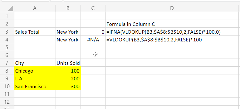
As you can see, since New York is not in the list an #N/A is triggered, the first version of the formula returns a 0 which we could then use in our workbook if we need to.

Trap every error?

As you’re building your workbook consider the effects of trapping the error versus knowing there is an error. Sometimes we want to see the error, to know that the workbook is not working as we intended. For instance in the example above, we are returning 0 for cities not in the list, however since our worksheet is to tell us total sales $0 is also an acceptable answer. We have no easy way to tell if there were no sales in a city or that the city is not in the list, which might indicate a data issue.

This is a problem known in Computer Science as the semi predicate problem where an error can be confused as a valid value. To prevent this care must be used when selecting what errors we want to trap and which we want to allow to break the workbook.

Excel has a variety of error codes to help the user understand why their formula isn’t working. Excel also has useful formulas for trapping and resolving potential errors. Careful and considerate use of these can lead to well constructed and robust workbooks.

Do you want to learn how to automate your financial workpapers? Do you want to get started with VBA?

My book, Beginning Microsoft Excel VBA Programming for Accountants has many examples like this to teach you to use Excel to maximize your productivity! It’s available on Amazon, Apple iBooks and other eBook retailers!

Learn More:

Function pages on Microsoft Support

Microsoft Excel Date Functions Round Up

What day is it? What day will it be 10 months from now? How many days until the end of next month? Microsoft Excel has a wide variety of date functions. This article will focus on several of the most useful. Hopefully you’ll find a few to add to your function repertoire.

DATEVALUE

Excel stores dates in a serial number format. Serial number 1 represents January 1, 1900 and each day after that increments the serial number by one. In other words January 2nd 1900 is 2 and serial number 44074 is August 31, 2020. Most of the date functions require this serial number. If you want to work with a date in a common format such as 08/31/2020 DATEVALUE is your go to.

Usage is: = DATEVALUE(“date”)
Example: =DATEVALUE(“08/31/2020”) will result in its serial 44074

Note: For the examples in this article, we’ll use DATEVALUE in place of a date serial

EOMONTH

EOMONTH results in the last day of a given number of months. I wrote an entire post on it here already showing a use case in accrual accounting. You can read that post here.

Excel EOMONTH Function Leads to Consistent Expense Accruals

Usage is: =EOMONTH([DateSerial], [number of months])
Example: =EOMONTH(DATEVALUE(“08/05/2020”),0) results in 08/31/2020

EDATE

EDATE results in a date that is the specified number of months before or after the given start date. Use negative numbers to give prior months and positive values for future ones.

Usage is:=EDATE([start date], [number of months])
Example: if we want the following month =EDATE(TODAY(),1) or if we want the day one month prior =EDATE(Today(),-1)

TODAY

TODAY() results in today’s date, it can be used as a parameter in formulas that need a date and we’ll use it in many of the following examples.

Usage: =TODAY()
Example: to get today’s date =TODAY()

DAYS

DAYS results in the number of days between two dates, excluding the end date. Unlike other date functions you can provide a date in a text format as a parameter. Although it won’t hurt any if you use DATEVALUE, a serial date or even TODAY()

Usage: =DAYS([end date],[start date])

Example: to get the number of days between August 1st and August 10th =DAYS(“8/10/20”,”8/1/20”)

WORKDAY.INTL

WORKDAY.INTL results in the date that’s the number of weekdays away from the given start date. This version of the WORKDAY function allows finer control over weekends and holidays than the vanilla WORKDAY function. The weekend day combinations are listed in a table that can be found on Microsoft’s support page (links in the Learn More section at bottom). If the weekends parameter is omitted, the default weekend is Saturday & Sunday.

Usage: =WORKDAY.INTL([start date], [number of days, [weekends], [holidays])
Example: To get a day 5 workdays prior to August 1, 2020 where Wednesday is the only day considered a weekend: =WORKDAY.INTL(DATEVALUE(“08/01/2020”),-5,14)

YEARFRAC

YEARFRAC results In the fractional portion of a year that has(will) elapse between two dates

Usage: =YEARFRAC([start date], [End date])
Example:To see what portion of the year passes between January 1st and June 30th (i.e. 0.50) =YEARFRAC(DATEVALUE(“01/01/2020”),DATEVALUE(“06/30/20”))

WEEKDAY

WEEKDAY Results in a number which translates in the day of the week of the provided date.

A Result of 1 is Monday and 7 is Sunday the other numbers between Correspond to each successive day

Usage: =WEEKDAY([date])
Example: to find which day of the week (i.e. 7 which is Sunday) =WEEKDAY(DATEVALUE(“08/01/20”))

Extract functions

The next three are what I call the extract functions because they allow you to extract or single out a part of the given date.

DAY

DAY Results in the day portion of a given date. This formula is useful for extracting the day data when needed.

Usage:=DAY([date])
Example: to get the 1 out of August 1, 2020 =DAY(DATEVALUE(“08/01/2020”))

MONTH

Month results in the month portion of a given date. This formula is useful for extracting the month data when needed.

Usage: =MONTH([date])
Example: to get 8 (for August) out of August 1, 2020 =MONTH(DATEVALUE(“08/01/2020”))

YEAR

YEAR results in the year from a given date. This formula is useful but you need to extract the year from a given date.

Usage: =YEAR([date])
Example: to get 2020 out of August 1, 2020 =YEAR(DATEVALUE(“08/01/2020”))

Want to learn how to automate your financial workpapers? Do you want to get started with VBA?

Learn More:

Function pages on Microsoft Support:

Example Workbook can be found at: MicroSoft OneDrive

Automate Formula Auditing in Microsoft Excel with FORMULATEXT

Technology: Office 365 as of July 2020

88% of spreadsheets have formula mistakes. A 2008 study by Havard economics found that many spreadsheets have significant calculation errors hidden within. The best way to avoid becoming a statistic is through diligent review. FORMULATEXT is a function that will help automate a diligent review of our workbooks.

FORMULATEXT is an Excel function that results in the formula of the target cell.

It’s usage is:

=FORMULATEXT([target cell])

This result is the formula of the target cell, i.e. the contents of the formula bar.

This alone makes reviewing the formula easier since it’ll be visible in the grid. Let’s take this one step further. In the example below we will compare formulas to a known formula and see if there’s any differences.

In this example we want to add two numbers and ensure that a SUM formula is used instead of directly adding the cells together.

Columns A and B have values
Column C has a formula to add A & B together
Column D has the FORMULATEXT function to show us the calculation in C
Column E has a text version of the formula we wanted used To type a formula as text put a single quotation mark before the equal sign (i.e. ‘=D3-E3)
Column F is an equality formula to show us if they are the same

We can see that Row 3 is not using the correct formula since there’s a False result in cell F4.

Here’s a real world example worksheet. This is a basic real estate escalation calculation. The goal is to ensure the formulas that determine the amounts owed or refunded are correct.

The mechanics of this worksheet are:

Columns A – F have the escalation calculation for each of the 3 tenants in this property
The formula in Column F should be the difference between the escalations billed in column E and the amount of expenses eligible for recovery in column D
Column H has a FORMULATEXT function getting the contents of column F on that row
Column I has the correct formula as text. To type a formula as text put a single quotation mark before the equal sign (i.e. ‘=D3-E3)
Column J compares H and I (i.e. =H3=I3) and will result in TRUE if they are the same or FALSE if they are different. I added some conditional formatting to highlight FALSE results in red

The False result here tells us that the formula in F4 is not the one we are expecting.

Another potential use of FORMULATEXT of is in creating dynamic documentation of the workbook. For example a sheet can be designated as the reference of all formulas contained in the workbook and through the formula they can link to the calculation sheets.

These are simple examples, but one could build upon the ideas. Combined with cell protections one could build a very robust formula review app. With a simple review mechanism such as FORMULATEXT, Microsoft Excel can help us ensure we have reliable worksheets that keep our clients in the 12%

Want to learn how to automate your financial workpapers? Do you want to get started with VBA?

Learn More:
Link to example worksheet at OneDrive

FORMULATEXT Function: https://support.microsoft.com/en-us/office/formulatext-function-0a786771-54fd-4ae2-96ee-09cda35439c8

TEXTJOIN function makes list building easy

Technology: Office 365 as of 2020

Microsoft introduced a new function which makes combining the contents of cells even easier than before. In addition to concatenating, or joining, the contents of cells the TEXTJOIN function also allows you to insert a delimiter between each item. This makes it more powerful than the old concatenate formula.

The ability to add a delimiter is what makes this function very useful. In the past we had the CONCAT and CONCATENATE functions which would join together text however, depending on the application, you usually need some character between your values.

Here’s a common example. Pasting a list of email addresses from Excel into an email in Outlook. The application expects a semicolon or comma between each email address or name, however you may not have included these characters in the list in Excel as it wouldn’t make sense to store this with the data.

If you require functionality similar to the old CONCATENATE function you can set the delimiter to “” which joins the text together without any character between each item. There is also the ability to include or exclude blank cells in the cell range from the results. If you need to do this depends on your use case.

The syntax is =TEXTJOIN([delimiter], [ignore blank cells], [cell range])

Where:

Delimiter is any character you want between your list. The character need to be enclosed with quotes, i.e. “;” This is required.

Ignore blank cells is either True or False depending if you want blanks included in your list. This is required

And the cell range is your list items you’re wanting to join together. You can also have multiple ranges in this field if you need them.This is required.

Let’s look at some examples

This first example presents a case where we want to email some individuals, to put their email addresses in the To field of our email client we need them separated by a semi-colon.

This next example provides a result similar to the old concatenate function. In this example the list of numbers is joined together without any delimiter.

The TEXTJOIN function saves a lot of time for those of us who use Excel to work with data needed in other applications. The power of adding a delimiter means you can quickly transform a list stored in a cell range to suit the needs of your application. It’s a simple & powerful formula to add into your repertoire.

Do you want to get started with VBA? Want to learn how to automate your financial workpapers?

Learn More:

Example Workbook:View Workbook on Microsoft OneDrive

TextJoin Function: TEXTJOIN at Microsoft Office Support

N Function Allows for Documentation in Excel’s Formula Bar

Microsoft Excel’s N function has many uses, including Switching and in line documentation

We commonly use Excel’s comment or note function to explain formulas or where the cell values come from. But, have you ever wanted to put this information in the formula bar itself? Sometimes it’s more helpful to document our formulas and data right where the user is reading them. Enter Excel’s N function.

The N function converts it’s parameter to a number. This is not to be confused with the VALUE function which converts text to number values. The N function will convert any text given to it to the value zero. If that doesn’t sound useful, keep in mind the additive property of zero anything added to zero is the original value. With this in mind, you can use this function to insert comments into the formula. For example if you had a formula to give an annual average and increase it by 3% your formula might be =AVERAGE(A1:A12)*1.03+N(“Returns a 3% increase in the average”). This use is shown in the featured image.

Switching in Formulas

Another interesting property of the N function is the way it converts TRUE or FALSE values. N will return the value 1 for a TRUE or 0 for a FALSE. Considering the multiplicative properties of 1 and 0 we can use this to create switches in our formula. A switch is where an operation is included in the final result if it’s multiplied by 1. For Example, this formula would result in the value 2 =(2*N(FALSE))+(2*N(TRUE)) if you expanded it it would be (2 x 0) + (2 x 1), change the first FALSE to TRUE and the value will increase to 4. With some careful workbook design, the N function can be used to replace nested IF statements which would serve a similar purpose. Let’s look at a more sophisticated example.

The sample workbook features quarter ending dates and the date of the current workpaper. By simply changing the workpaper date the Year To Date amortization updates appropriately. I’ve also used the comment N technique described earlier to demonstrate that use.

The N function is deceptively powerful. On the surface it would be easy to dismiss, but with a little ingenuity and careful workbook design it’ll allow you to simplify your workpapers and provide great documentation in the formula bar.

Do you want to get started with VBA? Want to learn how to automate your financial workpapers?

Download the sample workbook (Excel 2010 and higher):

N-Workbook-Example Download

Learn More:

https://support.office.com/en-us/article/n-function-a624cad1-3635-4208-b54a-29733d1278c9

Creating a Chart of Accounts from a General Ledger in Microsoft Excel using VBA

Recently I was given the task of extracting a chart of accounts (COA) from a general ledger report. There are many ways I could have done this. Using Auto Filter comes to mind. Being me, I chose to write a small program in Visual Basic for Applications (VBA). In this post I will walk you through the design and code of the program I made.

Design:

First we need to determine the goals for our output or in this case the chart of accounts. I needed a report with:

account number
account description

In the source file we see that the account number is in Column A and the account descriptions are in Column E. We also see that rows that begin with a number are the rows that have the account number/description. Since that’s all we need we’ll ignore everything else.

With that information we know that our solution will have to do the following:

find or determine the first and last rows on the source worksheet
examine each row in the source worksheet to see if it starts with a number
if it does start with a number then
take the account number and
take the account description and
write them to the destination sheet
lastly increment the row in the destination worksheet

It’s obvious that we need a loop in this case we’ll use a FOR loop to examine each row of the source worksheet. It’s also clear we’ll need an IF statement to determine if the first character of the row is a number or not.

Code:

 
Sub ExtractCOA()
 
    'This program will extract the chart of accounts from a Yardi 7
    'default General Ledger (analytics) report run to Excel 
    'Derek Harlan April 2018 - Licensed in the Public Domain 

    'Setup Object Variables for the worksheets 
    'src will be the Source worksheet 
    Dim src As Worksheet 
    'dest will be the Destination worksheet 
    Dim dest As Worksheet 
    'Setup some counter variables 
    'firstRow / lastRow will be the first and last rows of the Source workbook 
    'nextRow will be the row to write in the Destination workbook 
    'i will be the counter in the For loop 
    Dim startRow as Long 
    Dim lastRow As Long 
    Dim i As Long 
    Dim nextRow As Long 
    'Set the initial values for the variables 
    Set src = Sheets("Report1") 
    Set dest = Sheets("Sheet1") 
    startRow = 6 ' this is easy to determine so I just set it the row number 
   'Find the last row by searching the workbook from the bottom row up 
   'and assign it to the variable 
    lastRow = src.Range("A1048576").End(xlUp).Row 
    i = 0 
    nextRow = 2 'Row 1 will be the headers in the worksheet so Row 2 is where the data starts 
    'We'll loop through each row between the first and last rows of the Source workbook 
    For i = startRow To lastRow Step 1 
       'If the first character of the value of the cell in A and the current row (i) is a number then 
       'that row has the account number and name on it 
        If IsNumeric(Left(src.Range("A" & i).Value, 1)) Then 
            'set the values in the destination worksheet from the values on the 
            'current row of the source worksheet 
            dest.Range("A" & nextRow).Value = _ 
               src.Range("A" & i).Value 
            dest.Range("B" & nextRow).Value = _ 
               src.Range("E" & i).Value 
            'lastly increment the nextRow in the destination worksheet 
             nextRow = nextRow + 1 
        End If 
    Next i 
End Sub

Running it creates this output –

With both of the requirements met I can say this was a success!

This project took about 20 minutes, from start to finish. In this instance I’m not sure if I saved any time however should I need to do this again I already have the program ready. When evaluating alternatives think about how often you’ll be asked to do this. It may take time to come up with the initial program but once you have it, you see a colossal increase in productivity!

Do you want to get started with VBA? Or want to learn what a FOR loop is?

Check out my book for more uses of Excel VBA in your daily work:

Beginning Microsoft Excel VBA Programming for Accountants

available on Amazon, Apple iBooks and other eBook retailers!

Questions or comments? Connect with me on

Facebook https://www.facebook.com/DerekHarlanWriter/

Twitter https://twitter.com/tazbirdinvader