Stale Accrual Detector – CRE MicroApps vol. 1

A common financial review task is to identify and investigate expense accruals over a certain age. This helps us ferret out estimates that got stuck or maybe even items paid from another expense line. When a reviewer is tasked with dozens of reviews it can be easy to miss one and I though maybe a small app dedicated to identifying these would be beneficial.

Welcome to the first in a series of MicroApps, these will be small Python based apps that focus on one task. This comes from the Linux mehodology of make one application that does one thing really well. In this series we’ll build several applications dedicated to a sole function. This will allow the user to build a toolkit which they can depoly in depening on the situation they are in.

One of the first challenges for this MicroApp is building a way for Python to find stale accruals. The General Ledger (GL) date is useless sine it will tend to be a date in the period, so the best key is to parse the description. Of course the application needs to be nimble enough to parse the string and find a meaningful date from it.

This project was written in Python 3 using the regex and Pandas modules to support it’s code. For this post we’ll keep this high level – if you’re interested in the code please let me know!

The goals for this application are to:

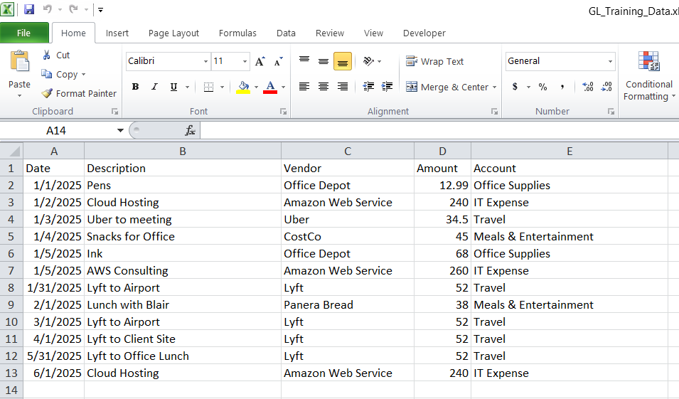
Read a GL export
extracts the intended accrual period from the description
compares it to the current period
flags stale accruals
includes property numbers (because CRE always needs property context)
run from a simple command‑line interface

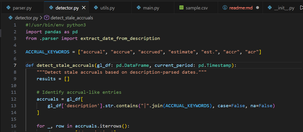
Even though this is a small tool, I organized it like a real Python project. Each file has one job, which keeps the code clean, readable, and easy to extend as I build more MicroApps.

The project files for the Stale Accrual Checker

These are the program files I’ve created and their purpose:

parser.py	Extracts dates from messy GL descriptions using regex patterns. This is where the “intelligence” of the tool lives.
detector.py	Applies the stale‑accrual logic. It takes the parsed dates, compares them to the current period, and assigns a status like ok, warning, or stale.
utils.py	Handles loading the GL file into a DataFrame. This will become reusable across future tools.
main.py	The command‑line interface. This is the file you run to execute the tool.
__init__.py	An empty file that tells Python, “This folder is a package.” Without it, the imports between these files wouldn’t work. This structure might look like overkill for a tiny script, but it sets me up to reuse pieces of this project in future micro‑apps — and it teaches beginners how real Python projects are organized.

How the Tool Works

The logic is simple:

Load the GL file
Identify accrual‑like entries (based on keywords)
Extract a date from the description
Normalize it into a real period end date
Compare it to the current period
Flag anything older than 60–90 days

This is the kind of problem where regex shines — descriptions are messy, but they follow patterns.

The Parser (`parser.py`)

This file looks for patterns like:

MM/DD/YY
MM/YYYY
MM-YYYY
September 25
Sep 2025

It returns a real datetime object representing the period.

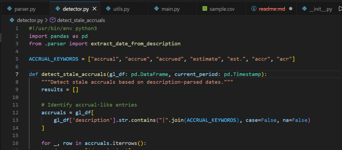
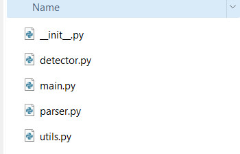
The Detector (`detector.py`)

This file:

filters for accrual‑like descriptions
applies the parser
calculates age in days
assigns a status
includes the property number in the output

The output is a clean DataFrame you can export, filter, or drop into a report.

Running the Tool

From the parent directory of the project:

python -m StaleAccrualChecker.main gl.csv --current 2025-12-31

This prints a table of stale accruals, including:

property number
description
amount
parsed period
age in days
status

Example:

property_number	description	amount	parsed_period	age_days	status
1001	04/2025 Window Cleaning Accrual	4500	2025‑04‑30	210	stale

Closing

If you’ve ever stared at a GL description trying to guess how old an accrual really is… this tool is for you. It’s small, practical, and easy to extend — and it’s the perfect starting point for building a real accounting automation toolkit in Python.

Do you want to learn how to automate your financial workpapers? Do you want to build MicroApps like this one to bloster your own automation toolkit? Do you want to get started with VBA?

My book, Beginning Microsoft Excel VBA Programming for Accountants has many examples like this to teach you to use Excel to maximize your productivity! It’s available on Amazon,Apple iBooks and other eBook retailers!

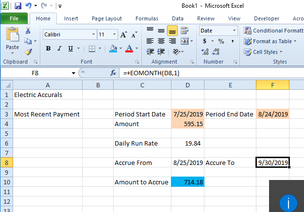
A Simple Python Machine Learning Script to help Accountants with Account Miscoding

With all the push for AI in the workplace I was curious if I could build a small program using machine learning to perform some useful function for accountants and financial reviewers – as account miscoding came to mind I wrote a program that would predict the account coding of a payable, this could aid a reviewer in determining if the months payable are coded correctly. I made a mock general ledger in Excel and trained a small machine learning model to predict which account each transaction should belong to. If the model’s prediction doesn’t match the coded account, that’s a potential miscoding.

A screenshot from Excel showing a mock general ledger for training data

This model was built in Python 3.9 using Pandas, scikit learn and a couple other modules to support transforming the Excel file into a model the program can work with.

What is Machine Learning

Machine learning is a subset of artificial intelligence that enables computers to learn and improve from experience without being explicitly programmed, by identifying patterns in data through algorithms trained on examples like labeled images or past transactions.

It works by feeding data into models, allowing predictions on new data. You see this everyday in recommendations for movies on streaming services, filtering spam emails, or detecting fraud in banking.

Machine learning is basically pattern recognition.

If your GL says:

“Office Depot – pens” → Office Supplies
“Printer ink” → Office Supplies
“AWS cloud hosting” → IT Expense
“Uber to client site” → Travel
“Lunch with client” → Meals

…then the model learns those patterns.

Give it a new transaction like:

“AWS EC2 monthly bill – Amazon Web Services – $260”

and it will say:

“This looks like IT Expense.”

If the GL has it coded as something else, that’s a red flag.

Here’s the Python code:

#! python3
#GL Classifer Bot

import pandas as pd
from sentence_transformers import SentenceTransformer
import numpy as np
from sklearn.ensemble import RandomForestClassifier
from sklearn.model_selection import train_test_split

df = pd.read_excel(r"C:\GL_Training_Data.xlsx")

# Load a lightweight embedding model
model = SentenceTransformer("all-MiniLM-L6-v2")

# Combine text fields into one string
df["text"] = df["Description"].astype(str) + " " + df["Vendor"].astype(str)

# Convert text to embeddings
embeddings = model.encode(df["text"].tolist())
X = np.hstack([embeddings, df[["Amount"]].values])
y = df["Account"]

X_train, X_test, y_train, y_test = train_test_split(
    X, y, test_size=0.25, random_state=42
)

clf = RandomForestClassifier()
clf.fit(X_train, y_train)

def predict_account(description, vendor, amount):
    text = description + " " + vendor
    emb = model.encode([text])
    X_new = np.hstack([emb, [[amount]]])
    return clf.predict(X_new)[0]

print(predict_account("AWS EC2 monthly bill", "Amazon Web Services", 260.00))

the last line feeds in a transaction and the output is it’s expected coding.

A simple walkthrough

Here’s the workflow of how the application works:

1. I loaded my GL from Excel.

Just a simple table with:

Date
Description
Vendor
Amount
Account

2. I converted the text into “meaning vectors.”

This sounds fancy, but it’s basically a tool that turns text like:

“Uber to client site”

into a list of numbers that represent its meaning.

3. I trained a small model to learn the patterns.

It looks at:

the meaning of the description
the vendor
the amount
the account it was coded to

…and learns how they relate.

4. I asked it to predict the account for new transactions.

If the prediction doesn’t match the coded account, I flag it.

That’s it. No deep learning, no giant datasets, no complicated math.

The output with a box drawn around the predicted account

What surprised me

When I only had 8 rows of data, the model predicted everything as “Office Supplies.”
Once I added a few more rows — it suddenly started predicting correctly.

That’s the magic of small ML models: they don’t need much to start learning.

Why this matters for accountants

This tiny example shows how machine learning can help with:

miscoded expense detection
reclass suggestions
anomaly spotting
cleaning up messy GLs
speeding up month‑end review

And you can build the whole thing in under an hour.

The takeaway

Machine learning doesn’t have to be intimidating.
You can start with:

a tiny GL
a few lines of Python
and a simple idea:
“Does this transaction look like the account it was coded to?”

That’s enough to demonstrate the concept — and enough to spark ideas for real‑world automation. This could easily be expanded to use a more complicated general ledger and to automatically search a general ledger under review for correct coding.

Do you want to learn how to automate your financial workpapers? Do you want to get started with VBA?

Excel Functions for Financial Reviewers

For those of us who review accounting workbooks it’s helpful to have a few tools to make the review easier. In today’s blog post I’m going to list 3 of my favorite Excel formulas or shortcuts that improve the quality of my reviews.

View Formulas helps you remove plugs or audit formulas

Pressing control and the tilde key (i.e. CTRL + ~) will change Excel to show the formulas in each cell rather than the values. This is very helpful when reviewing workbooks to ensure there are no plug values and that the formulas are consistent have the right ranges, etc. Press CTRL + ~ to put the view back to normal

The shortcut key CTRL + ~ changes the cells to show their formula rather than the value

As you can see in the screenshot, with view formulas it’s very easy to spot formula inconsistencies.

TEXTJOIN for making lists

The TEXTJOIN formula allows you to create lists easily with a seperator character. This is particulatly useful in my trade for combining lists of entites to put into a filter in the accounting system. The syntax of TEXTJOIN is = TEXTJOIN (delimiter, Ignore Empty, cell range)

The delimiter is the character you want to separate the items with, it can be anything but I’ll use the carrot ^ character for this example.

Ignore Empty parameter is either TRUE of FALSE, normally you’ll use TRUE so that it doesn’t conisder any empty cells in the range.

In the screenshot below, you can see how I used the formula to easily create the list (i.e. propert1^property2^property3^property4)

SUMIFS for totaling by category

The SUMIFS formula is very handy to get a quick total. It’s syntax is

=SUMIFS(sum range, category range 1, category, [more categories])

The sum range is the values you want to add.

The category range is the labels for each value

The category is which label you want to add

Consider this example. We have two projects TI Project #1 and #2. If we want to add TI Project #1 interdependently we can do this very easily using the SUMIFS like this:

SUMIFS can easily add up categories for your review

Although we tend to look to excel functions for preparation, even reviewers can harness the power of Excel shortcuts and formulas to make them better reviewers and help reduce or eliminate errors.

Do you want to learn how to automate your financial workpapers? Do you want to get started with VBA?

Resources:

TEXTJOIN https://support.microsoft.com/en-us/office/textjoin-function-357b449a-ec91-49d0-80c3-0e8fc845691c

SUMIFS https://support.microsoft.com/en-us/office/sumifs-function-c9e748f5-7ea7-455d-9406-611cebce642b

Excel Error and Error Handling Roundup

Excel Error and Error handling Roundup

Technology used: Office 365, Excel 2021

You just typed the closing parentheses of that powerful lookup formula that’s going to save you hours next month on the report. You slowly depress the Enter key while feeling empowered as if the Excel gods have chosen you! Feeling the click your stomach turns as you watch the fire bestowed upon you turn into a ball of steam that wisps away. Excel is taunting you. Instead of the sales figures, you see #N/A but what could be wrong?

Excel’s formula errors are unpleasant to see but they’re trying to help us improve our spreadsheet game. In this article, we’ll learn about the types of formula errors that Excel will display, a few formulas to help us avoid them and some thoughts on good use of error trapping.

What are formula errors

Formula errors are the result that Excel returns when it is unable to evaluate and provide a proper answer to the formula in the cell. The errors always begin with a number sign (i.e. #) and then a word to give you a clue as to what is causing the error. Below is a table listing common errors and some of their causes

Error (As shown in the cell)	Description
#N/A	Commonly found in lookup formulas (e.g. Vlookup, Hlookup, Index, Match, etc) if the formula is unable to find what the formula is looking for
#VALUE!	Excel’s general error. Simply put, something is wrong with the formula.
#REF!	A cell reference is invalid, typical if you delete a row/column that was being referenced by the formula
#DIV/0!	Division by zero. The result of which is undefined mathematically.
#NUM!	Mathematical operations are being applied to non-numeric cells. You can force text to be treated as numbers using the VALUE() function.
#NAME?	Excel doesn’t recognize the formula name, usually the result of a typo (e.g. =SMU(A1:A5) instead of =SUM(A1:A5)
#NULL!	The range is not constructed correctly in the formula’s parameters (e.g A5 B7 instead of A5:B7)
#SPILL!	Excel is unable to return the results because there isn’t enough room. For example a FILTER function is returning 10 results but there are only 9 blank cells available

Microsoft Excel’s Formula Errors

What formulas can be used to stop errors?

Excel gives us two formulas to handle or trap errors. Using these formulas can make your worksheet more robust and user friendly. They can also allow your workbook to function despite Excel being unable to calculate a cell.

IFError

The IFError function allows you to provide an alternate value or formula if Excel encounters any of these errors: #N/A, #VALUE!, #REF!, #DIV/0!, #NUM!, #NAME?, or #NULL!.

Its usage is:

=IFError(cell reference or formula, value if error)

The cell reference is any cell or formula that you are testing to see if it has or results in an error.

The value if error is what will result if there is an error. Here you can be really creative. A common usage would be a helpful error message consider something like:

=IfError(1/0, “Division by zero is undefined”)

In this case the formula 1/0 (e.g. One divided by 0) would result in #DIV/0!, we can replace that with the more friendly error message explaining that we can’t divide a number by zero.

But you can also use a substitute formula. For example:

=IFError(1/0, A1/B1)

This formula will result in the value of cell A1 divided by B1. Coincidently if the values of A1 divided by B1 would result in an error, then that error will be displayed.

Using the IFERROR formula gives us a lot of flexibility in trapping and resolving errors.

IFNA

IFNA works very similar to IFERROR except it only works with the #N/A error. Otherwise it’s usage is identical. Recall from the table above that the #N/A error is only encountered with lookup formulas thus this formula will only trap cases where the lookup value can’t be found in the table.

Its usage is:

=IFNA(Cell Reference or Formula, value if error)

For instance:

=IFNA(Vlookup(A1,A2:B20,2,FALSE),”Value was not found”)

Would display Value was not found instead of #N/A if the lookup value couldn’t be found.

Similar to IFERROR you can use a formula or value in place of the value if error parameter, this can help keep the logic of your workbook functioning.

Consider this example:

A Vlookup function encapsulated by an IFNA function

As you can see, since New York is not in the list an #N/A is triggered, the first version of the formula returns a 0 which we could then use in our workbook if we need to.

Trap every error?

As you’re building your workbook consider the effects of trapping the error versus knowing there is an error. Sometimes we want to see the error, to know that the workbook is not working as we intended. For instance in the example above, we are returning 0 for cities not in the list, however since our worksheet is to tell us total sales $0 is also an acceptable answer. We have no easy way to tell if there were no sales in a city or that the city is not in the list, which might indicate a data issue.

This is a problem known in Computer Science as the semi predicate problem where an error can be confused as a valid value. To prevent this care must be used when selecting what errors we want to trap and which we want to allow to break the workbook.

Excel has a variety of error codes to help the user understand why their formula isn’t working. Excel also has useful formulas for trapping and resolving potential errors. Careful and considerate use of these can lead to well constructed and robust workbooks.

Do you want to learn how to automate your financial workpapers? Do you want to get started with VBA?

Learn More:

Function pages on Microsoft Support

Microsoft Excel Date Functions Round Up

What day is it? What day will it be 10 months from now? How many days until the end of next month? Microsoft Excel has a wide variety of date functions. This article will focus on several of the most useful. Hopefully you’ll find a few to add to your function repertoire.

DATEVALUE

Excel stores dates in a serial number format. Serial number 1 represents January 1, 1900 and each day after that increments the serial number by one. In other words January 2nd 1900 is 2 and serial number 44074 is August 31, 2020. Most of the date functions require this serial number. If you want to work with a date in a common format such as 08/31/2020 DATEVALUE is your go to.

Usage is: = DATEVALUE(“date”)
Example: =DATEVALUE(“08/31/2020”) will result in its serial 44074

Note: For the examples in this article, we’ll use DATEVALUE in place of a date serial

EOMONTH

EOMONTH results in the last day of a given number of months. I wrote an entire post on it here already showing a use case in accrual accounting. You can read that post here.

Excel EOMONTH Function Leads to Consistent Expense Accruals

Usage is: =EOMONTH([DateSerial], [number of months])
Example: =EOMONTH(DATEVALUE(“08/05/2020”),0) results in 08/31/2020

EDATE

EDATE results in a date that is the specified number of months before or after the given start date. Use negative numbers to give prior months and positive values for future ones.

Usage is:=EDATE([start date], [number of months])
Example: if we want the following month =EDATE(TODAY(),1) or if we want the day one month prior =EDATE(Today(),-1)

TODAY

TODAY() results in today’s date, it can be used as a parameter in formulas that need a date and we’ll use it in many of the following examples.

Usage: =TODAY()
Example: to get today’s date =TODAY()

DAYS

DAYS results in the number of days between two dates, excluding the end date. Unlike other date functions you can provide a date in a text format as a parameter. Although it won’t hurt any if you use DATEVALUE, a serial date or even TODAY()

Usage: =DAYS([end date],[start date])

Example: to get the number of days between August 1st and August 10th =DAYS(“8/10/20”,”8/1/20”)

WORKDAY.INTL

WORKDAY.INTL results in the date that’s the number of weekdays away from the given start date. This version of the WORKDAY function allows finer control over weekends and holidays than the vanilla WORKDAY function. The weekend day combinations are listed in a table that can be found on Microsoft’s support page (links in the Learn More section at bottom). If the weekends parameter is omitted, the default weekend is Saturday & Sunday.

Usage: =WORKDAY.INTL([start date], [number of days, [weekends], [holidays])
Example: To get a day 5 workdays prior to August 1, 2020 where Wednesday is the only day considered a weekend: =WORKDAY.INTL(DATEVALUE(“08/01/2020”),-5,14)

YEARFRAC

YEARFRAC results In the fractional portion of a year that has(will) elapse between two dates

Usage: =YEARFRAC([start date], [End date])
Example:To see what portion of the year passes between January 1st and June 30th (i.e. 0.50) =YEARFRAC(DATEVALUE(“01/01/2020”),DATEVALUE(“06/30/20”))

WEEKDAY

WEEKDAY Results in a number which translates in the day of the week of the provided date.

A Result of 1 is Monday and 7 is Sunday the other numbers between Correspond to each successive day

Usage: =WEEKDAY([date])
Example: to find which day of the week (i.e. 7 which is Sunday) =WEEKDAY(DATEVALUE(“08/01/20”))

Extract functions

The next three are what I call the extract functions because they allow you to extract or single out a part of the given date.

DAY

DAY Results in the day portion of a given date. This formula is useful for extracting the day data when needed.

Usage:=DAY([date])
Example: to get the 1 out of August 1, 2020 =DAY(DATEVALUE(“08/01/2020”))

MONTH

Month results in the month portion of a given date. This formula is useful for extracting the month data when needed.

Usage: =MONTH([date])
Example: to get 8 (for August) out of August 1, 2020 =MONTH(DATEVALUE(“08/01/2020”))

YEAR

YEAR results in the year from a given date. This formula is useful but you need to extract the year from a given date.

Usage: =YEAR([date])
Example: to get 2020 out of August 1, 2020 =YEAR(DATEVALUE(“08/01/2020”))

Want to learn how to automate your financial workpapers? Do you want to get started with VBA?

Learn More:

Function pages on Microsoft Support:

Example Workbook can be found at: MicroSoft OneDrive

Automate Formula Auditing in Microsoft Excel with FORMULATEXT

Technology: Office 365 as of July 2020

88% of spreadsheets have formula mistakes. A 2008 study by Havard economics found that many spreadsheets have significant calculation errors hidden within. The best way to avoid becoming a statistic is through diligent review. FORMULATEXT is a function that will help automate a diligent review of our workbooks.

FORMULATEXT is an Excel function that results in the formula of the target cell.

It’s usage is:

=FORMULATEXT([target cell])

This result is the formula of the target cell, i.e. the contents of the formula bar.

This alone makes reviewing the formula easier since it’ll be visible in the grid. Let’s take this one step further. In the example below we will compare formulas to a known formula and see if there’s any differences.

In this example we want to add two numbers and ensure that a SUM formula is used instead of directly adding the cells together.

Columns A and B have values
Column C has a formula to add A & B together
Column D has the FORMULATEXT function to show us the calculation in C
Column E has a text version of the formula we wanted used To type a formula as text put a single quotation mark before the equal sign (i.e. ‘=D3-E3)
Column F is an equality formula to show us if they are the same

We can see that Row 3 is not using the correct formula since there’s a False result in cell F4.

Here’s a real world example worksheet. This is a basic real estate escalation calculation. The goal is to ensure the formulas that determine the amounts owed or refunded are correct.

The mechanics of this worksheet are:

Columns A – F have the escalation calculation for each of the 3 tenants in this property
The formula in Column F should be the difference between the escalations billed in column E and the amount of expenses eligible for recovery in column D
Column H has a FORMULATEXT function getting the contents of column F on that row
Column I has the correct formula as text. To type a formula as text put a single quotation mark before the equal sign (i.e. ‘=D3-E3)
Column J compares H and I (i.e. =H3=I3) and will result in TRUE if they are the same or FALSE if they are different. I added some conditional formatting to highlight FALSE results in red

The False result here tells us that the formula in F4 is not the one we are expecting.

Another potential use of FORMULATEXT of is in creating dynamic documentation of the workbook. For example a sheet can be designated as the reference of all formulas contained in the workbook and through the formula they can link to the calculation sheets.

These are simple examples, but one could build upon the ideas. Combined with cell protections one could build a very robust formula review app. With a simple review mechanism such as FORMULATEXT, Microsoft Excel can help us ensure we have reliable worksheets that keep our clients in the 12%

Want to learn how to automate your financial workpapers? Do you want to get started with VBA?

Learn More:
Link to example worksheet at OneDrive

FORMULATEXT Function: https://support.microsoft.com/en-us/office/formulatext-function-0a786771-54fd-4ae2-96ee-09cda35439c8

TEXTJOIN function makes list building easy

Technology: Office 365 as of 2020

Microsoft introduced a new function which makes combining the contents of cells even easier than before. In addition to concatenating, or joining, the contents of cells the TEXTJOIN function also allows you to insert a delimiter between each item. This makes it more powerful than the old concatenate formula.

The ability to add a delimiter is what makes this function very useful. In the past we had the CONCAT and CONCATENATE functions which would join together text however, depending on the application, you usually need some character between your values.

Here’s a common example. Pasting a list of email addresses from Excel into an email in Outlook. The application expects a semicolon or comma between each email address or name, however you may not have included these characters in the list in Excel as it wouldn’t make sense to store this with the data.

If you require functionality similar to the old CONCATENATE function you can set the delimiter to “” which joins the text together without any character between each item. There is also the ability to include or exclude blank cells in the cell range from the results. If you need to do this depends on your use case.

The syntax is =TEXTJOIN([delimiter], [ignore blank cells], [cell range])

Where:

Delimiter is any character you want between your list. The character need to be enclosed with quotes, i.e. “;” This is required.

Ignore blank cells is either True or False depending if you want blanks included in your list. This is required

And the cell range is your list items you’re wanting to join together. You can also have multiple ranges in this field if you need them.This is required.

Let’s look at some examples

This first example presents a case where we want to email some individuals, to put their email addresses in the To field of our email client we need them separated by a semi-colon.

This next example provides a result similar to the old concatenate function. In this example the list of numbers is joined together without any delimiter.

The TEXTJOIN function saves a lot of time for those of us who use Excel to work with data needed in other applications. The power of adding a delimiter means you can quickly transform a list stored in a cell range to suit the needs of your application. It’s a simple & powerful formula to add into your repertoire.

Do you want to get started with VBA? Want to learn how to automate your financial workpapers?

Learn More:

Example Workbook:View Workbook on Microsoft OneDrive

TextJoin Function: TEXTJOIN at Microsoft Office Support

N Function Allows for Documentation in Excel’s Formula Bar

Microsoft Excel’s N function has many uses, including Switching and in line documentation

We commonly use Excel’s comment or note function to explain formulas or where the cell values come from. But, have you ever wanted to put this information in the formula bar itself? Sometimes it’s more helpful to document our formulas and data right where the user is reading them. Enter Excel’s N function.

The N function converts it’s parameter to a number. This is not to be confused with the VALUE function which converts text to number values. The N function will convert any text given to it to the value zero. If that doesn’t sound useful, keep in mind the additive property of zero anything added to zero is the original value. With this in mind, you can use this function to insert comments into the formula. For example if you had a formula to give an annual average and increase it by 3% your formula might be =AVERAGE(A1:A12)*1.03+N(“Returns a 3% increase in the average”). This use is shown in the featured image.

Switching in Formulas

Another interesting property of the N function is the way it converts TRUE or FALSE values. N will return the value 1 for a TRUE or 0 for a FALSE. Considering the multiplicative properties of 1 and 0 we can use this to create switches in our formula. A switch is where an operation is included in the final result if it’s multiplied by 1. For Example, this formula would result in the value 2 =(2*N(FALSE))+(2*N(TRUE)) if you expanded it it would be (2 x 0) + (2 x 1), change the first FALSE to TRUE and the value will increase to 4. With some careful workbook design, the N function can be used to replace nested IF statements which would serve a similar purpose. Let’s look at a more sophisticated example.

The sample workbook features quarter ending dates and the date of the current workpaper. By simply changing the workpaper date the Year To Date amortization updates appropriately. I’ve also used the comment N technique described earlier to demonstrate that use.

The N function is deceptively powerful. On the surface it would be easy to dismiss, but with a little ingenuity and careful workbook design it’ll allow you to simplify your workpapers and provide great documentation in the formula bar.

Do you want to get started with VBA? Want to learn how to automate your financial workpapers?

Download the sample workbook (Excel 2010 and higher):

N-Workbook-Example Download

Learn More:

https://support.office.com/en-us/article/n-function-a624cad1-3635-4208-b54a-29733d1278c9

Excel EOMONTH Function Leads to Consistent Expense Accruals

The Excel EOMonth Function is a handy formula which will return a date representing the last day of a particular month. The month end date returned is determined by the second parameter.

The syntax is simple =EOMONTH(Start Date, Number of Months) where number of months can be positive or negative integer .

Any date can be used as a starting point in the first parameter. Regardless if it’s the first or thirtieth you’ll always get a date at the end of the month.

The second parameter is what makes the formula so interesting. You can specify the number of months to forward or backwards to return. To move backwards provide a negative number.

One potential use – would be to automate your monthly expense accruals. In the above sample workbook, the accountant only needs to update the most recent paid invoice. The formulas then automatically determine the period to accure.

The Accure From is simply the period end date plus one and then the EOMONTH in cell F8 determines the end of the following month. Using a formula like this would help you apply a consistent accrual methodology throughout your financials.

For more information on EOMONTH check out the official documentation https://support.office.com/en-us/article/eomonth-function-7314ffa1-2bc9-4005-9d66-f49db127d628

You can download the sample workbook below

EOMONTH Example Workbook Download

Microsoft Excel Date Functions Round Up – Derek Harlan on Excel EOMONTH Function Leads to Consistent Expense AccrualsAugust 5, 2020
[…] Excel EOMONTH Function Leads to Consistent Expense Accruals […]

Raspberry Pi Cooling Test

Dated: 8/1/2018 Technology/Software used: Raspberry Pi 3 Model B, Raspian Stretch (June 2018)

I’ve owned my Pi for a couple years now. I’ve always wanted to overclock it. Before you overclock you have to have a good cooling solution. I wanted to take this opportunity to test some various cooling solutions and talk about the process I went through. In this post I’ll explore my results from various cooling tests I conducted.

A word of caution: Overclocking your Raspberry Pi may void your warranty, do at your own risk. Due to differences in manufacturing some Pis may overclock well, some will not at all.
The following in no way is meant to be scientifically accurate testing and your results may very.

Why do I want to overclock? Well I sometimes use my Pi to run the RetroPie operating system. I enjoy retro gaming and I would love to be able to emulate N64 better. There’s a lot of mixed opinion and the general consensus is that the Pi is not fit for N64 emulation (spoiler alert: they’re right) but I wanted to try and see for myself if it was possible to play Goldeneye on my Pi.

Ultimately I wanted to use both a small 5 volt fan and heat sink. But I was interested in seeing the thermal performance of each component individually. I tested the heat and processor throttling of a stock configuration using the sysbench application. I was inspired by Christopher Barnett’s thermal tests on his YouTube channel – Explaining Computers and I used a similar bash script to test.

Moding the Case

My case, a very basic one for the Pi, wasn’t designed to hold a fan. I cut an opening and screw holes for the fan with a Dremel tool. You can see in the photos below the before and after. I hadn’t cut acrylic plastic before. I used a regular cutting disk for this. While it did the job, I noticed the plastic was getting a bit gummy which made it hard to control. I would have benefited form scoring the plastic before cutting. If I have to do this again, I’d try a different cutting disk and maybe first score the circle before cutting.

With the prep-work done I began the test. I tried five configurations, the Pi in the closed case (before cutting the fan hole), the Pi in an open case, the fan by itself, the heat sink by itself and finally both the heat sink and fan.

Before:

After:

Why is the cooling so important?

Running electrical components too hot can cause them to fail over time. Getting too hot in one instance can also cause an immediate failure. However, many modern computers have built in thermal protection which will reduce their power in an effort to cool the unit down. The Pi is no exception. Its thermal protection kicks in at about 80 C at this point the Pi will reduce it’s clock-speed to cool itself. I wanted to see how significant the throttling is. So I tracked both the average clock-speed throughout the entire test and the temperature between each test.

This is the script I had used. It’s a bash script which in Linux is like a batch file Windows. In other words a file which automatically runs a series of commands.

#! /bin/bash
echo "Baseline"
vcgencmd measure_temp
vcgencmd measure_clock arm
echo "Test 1"
sysbench --test=cpu --cpu-max-prime=20000 --num-threads=4 run >/dev/null 2>&1
vcgencmd measure_temp
vcgencmd measure_clock arm
echo "Test 2"
sysbench --test=cpu --cpu-max-prime=20000 --num-threads=4 run >/dev/null 2>&1
vcgencmd measure_temp
vcgencmd measure_clock arm
echo "Test 3"
sysbench --test=cpu --cpu-max-prime=20000 --num-threads=4 run >/dev/null 2>&1
vcgencmd measure_temp
vcgencmd measure_clock arm
echo "Test 4"
sysbench --test=cpu --cpu-max-prime=20000 --num-threads=4 run >/dev/null 2>&1
vcgencmd measure_temp
vcgencmd measure_clock arm
echo "Test 5"
sysbench --test=cpu --cpu-max-prime=20000 --num-threads=4 run >/dev/null 2>&1
vcgencmd measure_temp
vcgencmd measure_clock arm
echo "Complete"

The script will run the test five times. We’ll look at the specifics of the each command next, but in essence it displays a base line temperature and clock speed, then runs a stress test followed by displaying the temperature and clock-speed and repeats that sequence 5 times. I recorded the temperature and clock speed after each test into a LibreOffice Calc spreadsheet for analysis.

BASH Script commands

The line that begins with the #! is called a shebang or hash-bang. That identifies to Linux where the interpreter for the script is. In this case Linux will find BASH in my /bin/bash directory.

Next is the echo keyword. This keyword is similar to print() in Python. It will display the text between the quotes on screen. In this script it is used to indicate the beginning of each test. The echo keyword is useful to communicate with the user and let them know what’s going on within the script.

After that we have the commands that actually performs the stress test. Sysbench is a piece of software which is used to perform various benchmark test to determine performance. In this script, rather than gauge performance I am using the CPU benchmark to apply stress to the system which will cause it to generate more heat and I can see how effective my cooling solutions are. The parameters passed to the Sysbench utility are to test the CPU. The CPU test utilized by Sysbench is to determine all prime numbers bewteen 2 and max-prime number in this case 20,000. This is a very intensive task for the computer. I then sepcified that I wanted it to run on all four cores of the processor. Lastly I use the >/dev/null 2>&1 parameter to direct Sysbench’s output to NULL. In otherwords to disregard the results, because in this use case I don’t care what the efficencny of the processor is just it’s heat and clock-speed.

The next commands are two uses of the vcgencmd. Vcgencmd is a utility on the Raspberry Pi to display certain information. In this case I display two things: measure_temp which shows the system temperature and measure_clock arm which displays the current clock-speed of the ARM chip or the main microprocessor of the of the Raspberry Pi. The Raspberry Pi’s microprocessor normally runs at 600Mhz but can turbo up to 1.2Ghz if needed. If the Raspberry Pi gets too hot (around 80C), the system will reduce the speed in an effort to cool it down, this is called throttling. By checking the temperature and clock-speed I can see if the Pi is overheating and throttled slower.

Results

My prediction was that the Fan + Heat-sink would provide the best cooling, however I was surprised that the Fan by itself kept the Pi running near 70 C. I was also surprised that the heat-sinks I used (small aluminum ones) barley cooled the Pi below just having the lid off. We can also confirm from the data that the Fan + Heat-sink provided the best cooling keeping the Pi below 60 C.

From this graph we can see that the Pi only throttled while running without any cooling. The other cooling solutions were able to keep the Pi running at full speed (1200 MHz) throughout each test. From this test, I may have been able to get away with just a heat sink., however because I want to minimize the overall duration of heat exposure on my Pi so I will use both the Fan and the Heat-sink.

Conclusion

Testing the Pi in this way gave me some fascinating insights into different cooling options. In my testing I determined that using a Fan + Heat-sink offers the best cooling option and also does not lead to any throttling conditions. However, I was also able to determine that a Fan by itself offers a similar level of heat control.

Regrets

As I cautioned at the beginning this was not meant to be a scientific testing of different heat control methods. One thing in particular I would have like to have done was a real use case test of the thermal performance. My motivation was to improve the N64 emulation performance in RetroPie. I was able to find a stable overclock which various recommended as potentially useful for what I wanted to do. However, I’m sad to report that in my case it did not improve the performance, which as these same forums mentioned, may not because the nature of the Pi is just very different than an N64. Even though I was not able to improve the performance I’m still glad I was able to go through with this experience.

Want to learn more about Raspberry Pi? Well I haven’t written a book on that (yet) but if you are eager to learn Excel and VBA programming check out my book – Beginning Microsoft Excel VBA Programming for Accountants has many examples of automating Excel to teach you ways to maximize your productivity! It’s available on Amazon, Apple iBooks and other eBook retailers!

Questions or Comments?

Connect with me:

Facebook https://www.facebook.com/DerekHarlanWriter/

Twitter https://twitter.com/tazbirdinvader

How the Tool Works

The Parser (parser.py)

The Detector (detector.py)

Running the Tool

Closing

A simple walkthrough

1. I loaded my GL from Excel.

2. I converted the text into “meaning vectors.”

3. I trained a small model to learn the patterns.

4. I asked it to predict the account for new transactions.

What surprised me

Why this matters for accountants

The takeaway

Moding the Case

Why is the cooling so important?

BASH Script commands

Results

Conclusion

Regrets

The Parser (`parser.py`)

The Detector (`detector.py`)